Getting Started with Nucleus

Section 1: What is Nucleus?

Imagine you’re a machine learning engineer responsible for building a pedestrian detection algorithm. It’s easy to get started, perhaps by training a standard model on a small dataset. You get some preliminary results, and now you want to improve on the baseline. But what do you do next?

In academia, common approaches are new algorithms, different architectures, or larger hyperparameter searches. But academics fight with one hand tied behind their backs: they usually cannot edit their datasets. In practical applications, on the other hand, datasets are malleable and can be extended to suit a problem’s needs. In practice, the most effective way to improve an ML model is often to improve the dataset.

At Scale, we specialize in creating high-quality, large-scale training datasets for our customers. Expanding beyond our core strength of data labeling, we developed Nucleus because we think it should be easier to visualize, search, and improve computer vision datasets, and because we saw many ML engineers struggling to answer two core questions:

1. I know my ML model isn’t perfect. But where specifically does it fail today, and why?
2. How can I improve my dataset to fix these failures?

With Nucleus, ML teams can use their models to discover issues in their datasets, surface the part of the data distribution where models struggle most, compare model runs, and prioritize what new unlabeled data to label next.

In the rest of this post, we’ll walk through a step by step tutorial on how to get started with Nucleus. We’ll show you how to upload an image dataset with ground truth annotations, as well as how to integrate the Nucleus python client into a PyTorch training workflow to analyze model results.

Section 2: Getting Started with the Nucleus Python Client

The complete code for this tutorial is available in this colab notebook. If you’d like to follow along step by step and create a personal dataset on Nucleus, you will first need to make a free scale account and obtain a test API key. You can then copy the notebook and add your personal key to upload data for free.

To continue with the example of pedestrian detection, we’ll use the PennFudan pedestrian detection dataset to finetune a pre-trained Faster R-CNN model for a pedestrian detection task. PennFudan consists of 170 images labeled with both bounding boxes and segmentation masks. Some code has been omitted for brevity, see this colab notebook for the complete implementation. Let’s get started by instantiating the nucleus client and downloading the dataset.

Download the Dataset and Upload to Nucleus

1API_KEY = #YOUR SECRET API KEY HERE
2nucleus = nucleus.NucleusClient(API_KEY)

1%%shell
2# download the Penn-Fudan dataset
3wget https://www.cis.upenn.edu/~jshi/ped_html/PennFudanPed.zip .
4# extract it in the current folder
5unzip PennFudanPed.zip

To get started with Nucleus, we will first upload the PennFudan dataset to the Nucleus Dashboard. Uploading data is easy using the Nucleus python client — either specify the local file path or image url if your data is stored in the cloud. In this case, we’ve downloaded the PennFudan dataset locally, so for each dataset item we specify the file path of the image. We’ll use the file name as a reference_id that can be used to refer to the images in later API requests.

1nucleus_dataset = nucleus.create_dataset("PennFudan")
2DATASET_ID = nucleus_dataset.info()['dataset_id'] # Save unique ID for future use
3 
4def format_img_data_for_upload(img_dir: str):
5  """Instantiates a Nucleus DatasetItem for all images in the PennFudan dataset.
6    
7  Parameters
8  ----------
9  img_dir : str
10      The filepath to the image directory
11
12  Returns
13  ----------
14  List[DatasetItem]
15      A list of DatasetItem that can be uploaded via the Nucleus API
16  """
17  img_list = []
18  for img_filename in os.listdir(img_dir):
19      img_id = img_filename.split('.')[0]
20      item = DatasetItem(
21          image_location=os.path.join(img_dir, img_filename), 
22          reference_id=img_id,
23      )
24      img_list.append(item)
25  return img_list
26
27img_list = format_img_data_for_upload(IMG_DIR)
28
29response = nucleus_dataset.append(img_list)

Once the images are uploaded, the next step is to upload the ground truth bounding box annotations.

1def format_annotations_for_upload(annotations_dir: str):
2  """Instantiates a Nucleus BoxAnnotation for all ground truth annotations
3  in the PennFudan dataset.
4
5  Parameters
6  ----------
7  annotations_dir : str
8      The filepath to the directory storing mask annotations
9
10  Returns
11  -------
12  List[BoxAnnotation]
13      A list of BoxAnnotation items that can be uploaded via the Nucleus API
14  """
15  annotation_list = []
16  for mask_filename in os.listdir(annotations_dir):
17      img_filename = mask_filename.split(".")[0][:-5]
18      mask = Image.open(os.path.join(annotations_dir, mask_filename))
19      mask = np.array(mask)
20      boxes = get_boxes(
21          mask, use_height_width_format=True
22      ) 
23      for i in range(len(boxes)):
24          x = int(boxes[i][0])
25          y = int(boxes[i][1])
26          width = int(boxes[i][2])
27          height = int(boxes[i][3])
28          annotation = BoxAnnotation(
29              label=PEDESTRIAN_LABEL, 
30              x=x, 
31              y=y, 
32              width=width, 
33              height=height, 
34              reference_id=img_filename,
35          )
36          annotation_list.append(annotation)
37  return annotation_list
38
39annotations = format_annotations_for_upload(ANNOTATIONS_DIR)
40response = nucleus_dataset.annotate(annotations)

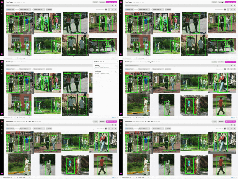
With the images and annotations uploaded, we can visualize the PennFudan Dataset in the Nucleus Dashboard.

From the insights tab, we can get a quick overview of the labeled dataset. In particular, you’ll notice that the annotations consist of exactly one class (pedestrian), and that the dataset overall is biased toward images with fewer annotations. The visualization, querying, and insights features in Nucleus make it easy to dig into interesting subsets of the training dataset.

Next, we’ll set up the Pytorch DataLoaders needed for training and evaluation.

Setting up transforms and DataLoaders

1def get_transform(train):
2transforms = []
3# converts the image, a PIL image, into a PyTorch Tensor
4transforms.append(T.ToTensor())
5if train:
6# during training, randomly flip the training images
7# and ground truth for data augmentation
8transforms.append(T.RandomHorizontalFlip(0.5))
9return T.Compose(transforms)
10# use our dataset and defined transformations
11dataset_train = PennFudanDataset('PennFudanPed', get_transform(train=True))
12dataset_test = PennFudanDataset('PennFudanPed', get_transform(train=False))
13# split the dataset in train and test set
14torch.manual_seed(1)
15N_TEST = 50
16indices = torch.randperm(len(dataset_train)).tolist()
17dataset_train = torch.utils.data.Subset(dataset_train, indices[:-N_TEST])
18dataset_test = torch.utils.data.Subset(dataset_test, indices[-N_TEST:])
19
20# define training and test data loaders
21data_loader = torch.utils.data.DataLoader(
22dataset_train, batch_size=2, shuffle=True, num_workers=0,
23collate_fn=utils.collate_fn)
24
25data_loader_test = torch.utils.data.DataLoader(
26dataset_test, batch_size=1, shuffle=False, num_workers=0,
27collate_fn=utils.collate_fn)

Use Slices to keep track of test and train sets within Nucleus

When evaluating model predictions, we’ll want to differentiate between train and test examples within the Nucleus platform. We can do so using slices. A slice is just a collection of dataset items. Below, we create slices for the train and test sets.

1get_slice_item_reference_ids(dataset: torch.utils.data.Subset):
2""" Given a Pytorch dataset, returns a list of reference_ids corresponding
3to the dataset's contents.
4
5Parameters
6----------
7dataset : str
8    A Pytorch dataset.
9
10Returns
11-------
12List[str]
13    A list of reference_ids for items to be uploaded to a Nucleus Slice.
14"""
15reference_ids = []
16for i in range(len(dataset)):
17    _, _, img_file_name = dataset[i]
18    ref_id = img_file_name.split(".")[0]  # remove file extension
19    reference_ids.append(ref_id)
20return reference_ids
21
22train_reference_ids = get_slice_item_reference_ids(dataset_train)
23slice_train = nucleus_dataset.create_slice(name='training_set', reference_ids=train_reference_ids)
24
25test_reference_ids = train_reference_ids = get_slice_item_reference_ids(dataset_test)
26slice_test = nucleus_dataset.create_slice(name='test_set', reference_ids=test_reference_ids)

Once a slice is created via the Python client, it will appear in the Nucleus interface. The slicing feature is useful for examining a particular subset of the dataset. When viewing a slice, the search bar queries are applied only to the items within the current slice.

Define the model & training loop

We are now ready to start using Nucleus to analyze experiments, the next step is to upload model predictions. In the code block below, we finetune the Faster R-CNN for 7 epochs before evaluating it on the test set consisting of 50 held-out examples.

In the code segment below, we’ve factored the details of the training loop into some helper functions imported from vision/references/detection/. Here’s the simplified training loop:

1get_model(num_classes):
2  # load an instance segmentation model pre-trained on COCO
3  model = torchvision.models.detection.fasterrcnn_resnet50_fpn(pretrained=True)
4  # get number of input features for the classifier
5  in_features = model.roi_heads.box_predictor.cls_score.in_features
6  # replace the pre-trained head with a new one
7  model.roi_heads.box_predictor = FastRCNNPredictor(in_features, num_classes)
8
9  return model
10
11  device = torch.device('cuda') if torch.cuda.is_available() else torch.device('cpu')
12  # our dataset has two classes only - background and person
13  num_classes = 2
14  # get the model using our helper function
15  model = get_model(num_classes)
16  # move model to the right device
17  model.to(device)
18  # construct an optimizer
19  params = [p for p in model.parameters() if p.requires_grad]
20  optimizer = torch.optim.SGD(params, lr=0.005,
21                              momentum=0.9, weight_decay=0.0005)
22  # and a learning rate scheduler which decreases the learning rate by
23  # 10x every 3 epochs
24  lr_scheduler = torch.optim.lr_scheduler.StepLR(optimizer,
25                                                 step_size=3,
26                                                 gamma=0.1)
27  # let's train it for 7 epochs
28  num_epochs = 7
29
30  model.train()
31  for epoch in range(num_epochs):
32  # train for one epoch, printing every 10 iterations
33  train_one_epoch(model, optimizer, data_loader, device, epoch, print_freq=20)
34  # update the learning rate
35  lr_scheduler.step()
36  # evaluate on the test dataset
37  evaluate(model, data_loader_test, device=device)

The evaluation output shows that overall, the finetuned model achieves an average precision of 0.827 and average recall of 0.386. Not bad for a first shot!

But now what? These summary statistics don’t tell us very much about how we could make this model better. That’s where Nucleus comes in. Below, we create a model_run, which functions as a container for the predictions from this experiment. Formatting the predictions and sending them to Nucleus takes just a couple lines of code, and can easily be integrated into a PyTorch evaluation function. Once these predictions are visible in the Nucleus dashboard, there are all kinds of error analysis tools at our disposal.

Adding model predictions to Nucleus

The first step for uploading model predictions is to create a Nucleus model. Below, we name the model fasterrcnn so that we can use it to track all experiments using this architecture.

1# Create a new model to track all of our Faster R-CNN experiments
2nucleus_model = nucleus.add_model(name="Pytorch Faster R-CNN", reference_id="faster_r_cnn")

Then, we create a corresponding modelrun. The modelrun will keep track of the results of this particular experiment. Once the modelrun object is created, we upload the modelpredictions.

1# Predictions for entire dataset
2def get_model_predictions(model, dataset):
3  """Gets bounding box predictions on provided dataset, returns
4  BoxPredictions that can be uplaoded to Nucleus via API
5
6  Parameters
7  ----------
8  model : 
9      Pytorch Faster R-CNN model
10  dataset :
11      Dataset on which to conduct inference.
12
13  Returns
14  -------
15  List[BoxPrediction]
16      A list of BoxPredictions that can be uploaded to Nucleus via API.
17  """
18  predictions = []
19  model.eval()
20  for i, (img, _, img_name) in enumerate(dataset):
21      pred = model([img.to(device)])
22      boxes = pred[0]["boxes"].cpu().detach().numpy()
23      img_id = img_name.split(".")[0]
24      for box in boxes:
25          (xmin, ymin, xmax, ymax) = box
26          x = int(xmin)
27          y = int(ymin)
28          width = int(xmax - xmin)
29          height = int(ymax - ymin)
30          curr_pred = BoxPrediction(
31              label=PEDESTRIAN_LABEL, 
32              x=x, 
33              y=y, 
34              width=width, 
35              height=height, 
36              reference_id=img_id
37          )
38          curr_pred = BoxPrediction(label=PEDESTRIAN_LABEL, x=x, y=y, 
39          width=width, height=height, reference_id=img_id)
40          predictions.append(curr_pred)
41  return predictions
42
43dataset_test_all = PennFudanDataset('PennFudanPed', get_transform(train=False))
44preds = get_model_predictions(model, dataset_test_all)
45
46model_run = nucleus_model.create_run(name="Faster R-CNN Object Detection (Finetuning)", dataset=nucleus_dataset, predictions=preds)

After model predictions are uploaded, we are ready to commit the model run. On commit, Nucleus automatically matches predictions to ground truth, calculates IoU, and indexes false positives and false negatives.

1model_run.commit()

Section 3: Analysis

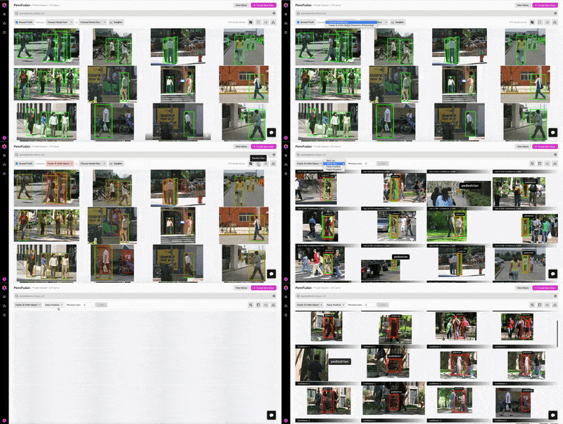
Now that we have the newly created model_run uploaded to the Nucleus platform, we can easily compare the predicted bounding boxes to the ground truth. Using the patches view, we can examine the individual predictions, sorting by best IoU, worst IoU, false positives, and false negatives.

In the patches view, we find a number of interesting observations:

Figure 1 (above): Examining false positives, we see that there are several instances where the model detected a cyclist as a pedestrian, but there was no ground truth bounding box for the cyclist. It would likely improve model performance to add a cyclist class; this would encourage the model to differentiate between the two types of objects, rather than just ignore cyclists.

Figure 2: The treatment of partially-occluded pedestrians is not consistent across different images. The occluded pedestrians are labeled in some places, but not in others.

Figure 3: There are many instances of missing ground truth annotations, particularly for pedestrians in the background.

Figure 4: In general, it seems the model performs best on pedestrians in the foreground, and exhibits poor performance on crowded images.

The worst-kept secret in machine learning

Nucleus shines a light on the worst-kept secret in machine learning: most datasets are filled with errors. Not only are they often full of bad annotations, but a typical ML engineer would never even notice. All we see is “average precision = 0.827”. Annotation errors are particularly insidious because they put a ceiling on model performance that is invisible to the ML engineer. The fact that these errors remain invisible is a failure of ML tooling. Nucleus helps address it. (In fact, one reason Scale can provide annotations at such high quality is because we leverage tools like Nucleus internally.)

Addressing the problem

Having the ability to visualize predictions and view errors all in one place gives us much better insight into what is actually going wrong with this model’s performance. Looking through the test set, we find that many of the predictions marked as false positives are actually just missing ground truth annotations. This is concerning — without high-quality labels on the test set, it’s difficult to trust evaluation metrics as an unbiased performance indicator.

Some actionable next steps we can take to improve this model’s performance are:

• Add a new label class for cyclist
• Correct missing annotations
• Source additional examples of crowded scenes

Correcting missing Annotations

In order to continue making progress on this pedestrian detection task, we need to be sure that the evaluation metrics on the test set are actually reflective of good model performance. We can only trust these metrics when the labels are exhaustive and high quality. Using Nucleus patches view, we correct missing annotations in both the train and test sets. The mean average precision (mAP) and mean average recall (mAR) from these experiments are summarized in the following table.

We found that evaluating the baseline model against the improved test set yields lower mAP and mAR, indicating that evaluating against noisy labels in the test set overestimated model performance. Moreover, after also correcting labels in the training dataset, the precision on the corrected test set improved by 7.98%, and recall improved by 7.36% relative to the baseline model. Overall, these results demonstrate that concentrating on label quality yields significant gains in overall performance.

Finding additional examples for the training dataset

One finding that label corrections do not address is the poor performance on crowded scenes. As discussed above, the dataset is heavily skewed towards examples with two or fewer pedestrians. Crowded scenes are rare in our dataset— one reliable way to address this edge case is to include more crowded scenes in our training dataset. In addition to the analysis tools like the patches and insights views, Nucleus supports a variety of features targeted at mining large sets of unlabeled data for rare scenarios.

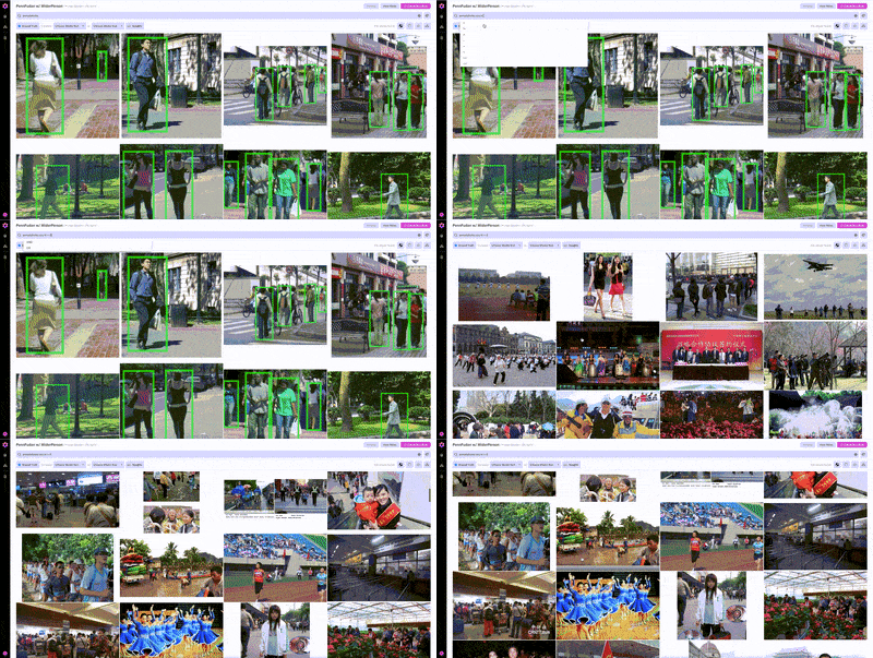
Since we’re already using all of the images in PennFudan for training and evaluation, we’ll use another publicly available dataset, WiderPerson, as a source of additional examples.

Putting PennFudan and WiderPerson together in one dataset, we now have a mix of labeled and unlabeled data.

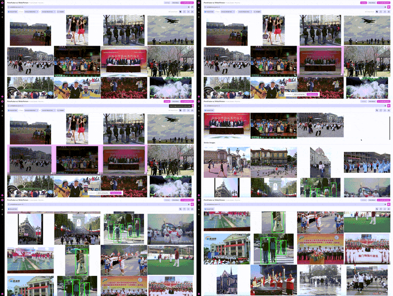
Once we’ve found one example from WiderPerson that we would want to include in our training set, we can use image similarity search to find other, similar examples.

Nucleus features like similarity search are particularly useful on massive datasets where it’s impossible to look through every example. Using similarity search, we can locate additional examples of pedestrians without having to rely on annotations, helping prioritize what unlabeled data to label next.

Conclusion

In this tutorial, we’ve demonstrated how Nucleus can help developers get actionable insights into model performance and dataset management. We’ve shown how to get started by uploading images, annotations, and predictions via the python API. Using Nucleus features for model analysis, we learned that labeling quality can really interfere with evaluation metrics. If such errors occur in small datasets like PennFudan, you can only imagine how commonly they occur in larger datasets like Imagenet and MSCOCO. Using Nucleus to identify issues with annotation taxonomy, quality, and consistency can thus play a huge role in producing quality results.

Acknowledgements

This tutorial is adapted from this PyTorch tutorial and uses the PennFudan Dataset.